# # Inverse design of a Y-branch using lumopt2
#
# An example of a parametric optimization for a Y-branch using lumopt2.
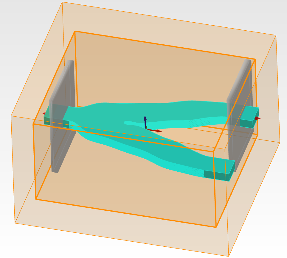
# This example demonstrates the use of a closed curve parametrization with a custom function to enforce symmetry.
# After the optimization, the final design is exported as a GDSII file.
#
# Prerequisites:
# - Valid Lumerical FDTD license with Lumerical 2026 R1.2 release or newer.
#
# ## Imports
# +
from pathlib import Path
from matplotlib import pyplot as plt
plt.ion()
import numpy as np
import ansys.lumerical.core as lumapi
import ansys.lumerical.core.lumopt2 as lmpt
# -
# ## Material, simulation, geometry
# ### Material and waveguide parameters
n_wg = np.sqrt(12.25) # Silicon refractive index
n_bg = np.sqrt(2.25) # Silicon oxide background
wg_width = 0.5e-6 # Waveguide width (500 nm)
wg_height = 0.22e-6 # Waveguide height (220 nm)
# ### Wavelength
# Set wavelength from 1300-1800nm
wavelengths = np.linspace(1300e-9, 1800e-9, 11)
# ### Design region parameters
splitter_span_x = 3.5e-6 # Length of the Y-branch splitter
wg_y_offset = 1.0e-6 # Output arm offset in y
port_width = 3 * wg_width # Port width to capture the mode
port_height = 2e-6 # Port height in z
fdtd_span_x = splitter_span_x + 0.8e-6
fdtd_span_y = 2 * wg_y_offset + 3 * wg_width
fdtd_span_z = wg_height + 2e-6
mesh_size = 25e-9
offset = 4 * mesh_size # Buffer between optimization region and FDTD edge
# ### Base simulation
def generate_base_sim(fdtd):
"""Build the FDTD region, the input/output ports, and the field monitor."""
fdtd.addfdtd(
{
"x": 0,
"x span": fdtd_span_x,
"y": 0,
"y span": fdtd_span_y,
"z": 0,
"z span": fdtd_span_z,
"index": n_bg,
"mesh accuracy": 3,
"mesh refinement": "precise volume average",
}
)
fdtd.addport({"name": "port_in"})
fdtd.set("injection axis", "x")
fdtd.set(
{
"direction": "Forward",
"x": -fdtd_span_x / 2 + 2e-7,
"y": 0,
"y span": port_width,
"z span": port_height,
"frequency dependent profile": False,
}
)
fdtd.addport({"name": "port_out1"})
fdtd.set("injection axis", "x")
fdtd.set(
{
"direction": "Backward",
"x": fdtd_span_x / 2 - 2e-7,
"y": wg_y_offset,
"y span": port_width,
"z span": port_height,
"frequency dependent profile": False,
}
)
# 2D field monitor through the device midplane (used by GraphicalVisualizer).
# Override the global monitor settings so this monitor only records the
# mid-O-band wavelength: that's all we need for live visualization and it
# keeps the monitor lightweight regardless of the optimization sweep.
center_wavelength = float(wavelengths[len(wavelengths) // 2])
fdtd.adddftmonitor(
{
"name": "field_monitor",
"x": 0,
"x span": fdtd_span_x,
"y": 0,
"y span": fdtd_span_y,
"z": 0,
"override global monitor settings": True,
"use source limits": False,
"frequency points": 1,
"wavelength center": center_wavelength,
"wavelength span": 0,
}
)
fdtd.setglobalsource("wavelength start", wavelengths[0])
fdtd.setglobalsource("wavelength stop", wavelengths[-1])
fdtd.setglobalmonitor("frequency points", len(wavelengths))
fdtd.setglobalmonitor("use wavelength spacing", True)
fdtd.setnamed("FDTD::ports", "override global monitor settings", False)
# ### Optimization region
# The optimization region is kept inside the FDTD bounds with a small buffer
optimization_region = lmpt.Box(
x_min=-splitter_span_x / 2,
x_max=splitter_span_x / 2,
y_min=-(wg_y_offset + wg_width),
y_max=wg_y_offset + wg_width,
z_min=-wg_height / 2.0,
z_max=wg_height / 2.0,
mesh_size=mesh_size,
)
# ### Closed curve geometry
# Closed-curve definition of the silicon Y-splitter. Walking the boundary
# counter-clockwise from the top-left, the four cubic segments (2, 6, 7, 11)
# form the parametric splitter region; everything else is fixed waveguide
# wall. Segments 2 and 11 control the outer walls of the upper / lower
# output arms (mirror partners across y=0); segments 6 and 7 control the
# inner V-shape between the two output arms (also mirror partners).
# +
path = [
lmpt.Segment([-fdtd_span_x / 2 - 200e-9, wg_width / 2], "linear"), # Segment 1
lmpt.Segment([-splitter_span_x / 2, wg_width / 2], "cubic"), # Segment 2 (upper outer wall, parametric)
lmpt.Segment([splitter_span_x / 2, wg_y_offset + wg_width / 2], "linear"), # Segment 3
lmpt.Segment([fdtd_span_x / 2 + 200e-9, wg_y_offset + wg_width / 2], "linear"), # Segment 4
lmpt.Segment([fdtd_span_x / 2 + 200e-9, wg_y_offset - wg_width / 2], "linear"), # Segment 5
lmpt.Segment([splitter_span_x / 2, wg_y_offset - wg_width / 2], "cubic"), # Segment 6 (upper inner wall, parametric)
lmpt.Segment([-splitter_span_x / 2 + 1500e-9, 0], "cubic"), # Segment 7 (lower inner wall, parametric)
lmpt.Segment([splitter_span_x / 2, -(wg_y_offset - wg_width / 2)], "linear"), # Segment 8
lmpt.Segment([fdtd_span_x / 2 + 200e-9, -(wg_y_offset - wg_width / 2)], "linear"), # Segment 9
lmpt.Segment([fdtd_span_x / 2 + 200e-9, -(wg_y_offset + wg_width / 2)], "linear"), # Segment 10
lmpt.Segment([splitter_span_x / 2, -(wg_y_offset + wg_width / 2)], "cubic"), # Segment 11 (lower outer wall, parametric)
lmpt.Segment([-splitter_span_x / 2, -wg_width / 2], "linear"), # Segment 12
lmpt.Segment([-fdtd_span_x / 2 - 200e-9, -wg_width / 2], "linear"), # Segment 13 (closes loop)
]
y_branch_curve = lmpt.ClosedCurve(path, z_min=-wg_height / 2, z_max=wg_height / 2, index=n_wg, optimization_region=optimization_region)
# -
# + [markdown]
# Check the geometry of the curve.
# The code will continue to run after this if the whole script is ran.
# -
# +
y_branch_curve.plot()
plt.pause(0.1)
# -
# ## Parametrization
# Parametrize the y-branch geometry and enforce mirror symmetry across y=0.
# Number of control vertices added on each parametric segment. Increasing
# these values gives the optimizer more shape freedom at the cost of more
# adjoint gradient evaluations per iteration.
# +
num_params_outer = 6
num_params_inner = 5
num_params = num_params_outer + num_params_inner + 1 # +1 for the V-tip x-offset
# -
# + [markdown]
# Subdivide the four cubic boundary segments. The mirror partners
# (11 mirrors 2, 7 mirrors 6) get the same number of vertices so the
# parametrization function below can pair them one-to-one.
# -
# +
split_result = y_branch_curve.split_segments(
[
lmpt.EqualSplit(segment_index=2, num_added_vertices=num_params_outer), # Upper outer wall
lmpt.EqualSplit(segment_index=6, num_added_vertices=num_params_inner), # Upper inner wall
lmpt.EqualSplit(segment_index=7, num_added_vertices=num_params_inner), # Lower inner wall (mirror of 6)
lmpt.EqualSplit(segment_index=11, num_added_vertices=num_params_outer), # Lower outer wall (mirror of 2)
]
)
seg2_vertices = split_result[2]
seg6_vertices = split_result[6]
seg7_vertices = split_result[7]
seg11_vertices = split_result[11]
center_vertex_idx = seg7_vertices[0] - 1 # V-tip vertex sits between segments 6 and 7
# -
# ### Defining the symmetric parametrization
# +
def symmetric_parametrization(params):
"""Enforce symmetric vertex displacements by mapping ``params`` to per-vertex deltas.
Enforces symmetric displacements in vertices by mapping vertex displacements
to the same parameter values in the ``params`` array. Uses the params
array as well as the vertex indices from earlier.
Parameters
----------
params : array-like
Length ``num_params`` array. Layout:
* ``params[0:num_params_outer]`` displace the outer-wall vertices
on segment 2 in +y; the mirror partners on segment 11 move in -y.
* ``params[num_params_outer:num_params_outer + num_params_inner]``
displace the inner-wall vertices on segment 6 in +y; the mirror
partners on segment 7 move in -y.
* ``params[-1]`` shifts the V-tip vertex in x.
Returns
-------
list of ParamVertex
Per-vertex displacement spec for every control vertex created by
``split_segments`` above.
"""
deltas = []
# Upper half
for i, idx in enumerate(seg2_vertices):
# Outer wall
deltas.append(lmpt.ParamVertex(idx=idx, delta_y=params[i]))
for i, idx in enumerate(seg6_vertices):
# Inner wall, starting at the end of the outer wall params
deltas.append(lmpt.ParamVertex(idx=idx, delta_y=params[num_params_outer + i]))
# V-tip vertex (x-only shift), this is the last parameter
deltas.append(lmpt.ParamVertex(idx=center_vertex_idx, delta_x=params[-1]))
# Lower half, traversed in reverse as we need the first vertex in segment 7 to pair with the last vertex in segment 6, etc.
# Symmetry enforced by making delta_y the negative of the same parameter
for i, idx in enumerate(seg11_vertices):
# Lower outer wall
mirror_i = num_params_outer - 1 - i
deltas.append(lmpt.ParamVertex(idx=idx, delta_y=-params[mirror_i]))
for i, idx in enumerate(seg7_vertices):
# Lower inner wall
mirror_i = num_params_inner - 1 - i
deltas.append(lmpt.ParamVertex(idx=idx, delta_y=-params[num_params_outer + mirror_i]))
return deltas
# -
# + [markdown]
# Bounds: the outer wall has more room to bow outward (positive y) than to
# bow inward (negative y). The inner wall and V-tip have asymmetric ranges
# tuned for the typical splitter optimization landscape.
# -
# +
bounds = (
[(-250e-9, 500e-9)] * num_params_outer + [(-400e-9, 200e-9)] * num_params_inner + [(-400e-9, 100e-9)] # V-tip x-offset
)
# -
# + [markdown]
# Call the parametrization function to apply the symmetric parametrization
# -
# +
y_branch_curve.set_parametrization_function(
func=symmetric_parametrization,
n_params=num_params,
bounds=bounds,
)
# + [markdown]
# Check the geometry again after applying parametrization.
# The code will continue to run after this if the whole script is ran.
# -
# +
y_branch_curve.plot()
plt.pause(0.1)
# -
# ## Figure of merit
# Define a broadband figure of merit: the target transmission to ``port_out1``
# is 0.5 (50% of the input power per output arm), averaged over the O-band
# sweep above. PNorm broadcasts the scalar target across all wavelengths
# automatically.
# +
port_out = lmpt.PortResults("port_out1", metric="transmission", wavelengths=wavelengths)
y_branch_fom = lmpt.Fom(port_out, fct=lmpt.PNorm(p=2, target=0.5))
# -
# ## Optimization session setup
# ### FDTD session
# Create an FDTD session with visible UI
fdtd_session = lmpt.FdtdSession(show_fdtd_cad=True)
# ### Project
# Create the project (FOM is defined in y_branch_setup.py)
# +
project = lmpt.Project(setup=generate_base_sim, parametrization=y_branch_curve, fom=y_branch_fom, fdtd_session=fdtd_session)
# -
# + [markdown]
# Uncomment and run the code below to validate that the parameter and project setup was done correctly
# -
# +
# params = project.parametrization.get_initial_params()
# lmpt.validate_gradient(project=project, params=params, perturbation=1e-9)
# -
# + [markdown]
# ### Optimizer
# Use SciPy's L-BFGS-B (gradient-based, supports bounds). The project's
# adjoint gradient turns each iteration into one forward + one adjoint sim,
# which is the same per-iteration cost as a gradient-free method but with
# much better convergence per iteration in the smooth-FOM regime.
# -
# +
optimizer = lmpt.ScipyOptimizer(method="L-BFGS-B", max_iter=30)
# -
# ### Visualizer
# Visualizer 1: FOM trace, gradient-norm trace, current geometry, and
# the real part of the Ey field so we can watch the splitter mode reshape
# during optimization.
# +
visualizer = lmpt.GraphicalVisualizer(
figsize=(12, 10),
layout=(2, 2), # Arrange panels in 2x2 grid
panels=[
lmpt.FomPanel(),
lmpt.GradientNormPanel(),
lmpt.GeometryPanel(),
lmpt.MonitorPanel(
monitor_name="FDTD::ports::port_out1",
result_name="expansion for port monitor.T_out",
operation="abs",
title="|T_out| (matches FOM)",
# Clamp the transmission trace to the physical
# [0, 1] range so the plot stays comparable
# iteration-to-iteration even when the
# baseline transmission starts very low.
# ``axes_kwargs`` is forwarded verbatim to
# ``ax.set(**axes_kwargs)``.
axes_kwargs={"ylim": (0.0, 1.0)},
),
],
)
# -
# + [markdown]
# Visualizer 2: Plot the y-direction electric field at the midplane monitor, for the midband wavelength.
# -
# +
visualizer2 = lmpt.GraphicalVisualizer(
filename_prefix="field_plot_Ey",
panels=[
lmpt.MonitorPanel(monitor_name="field_monitor", result_name="E.Ey", operation="real", title="Ey field (real part)"),
],
)
# -
# ### Optimization session
# Put everything together into an optimization session
optimization = lmpt.Optimization(
project=project,
optimizer=optimizer,
callbacks=[lmpt.FileLogger(), visualizer, visualizer2],
)
# ### Run optimization
result = optimization.run()
# + [markdown]
# The final visualizer is shown below
#
# The final electric field is shown below
#
# -
# ## Save project
best_params, best_fom = result
project.save_project("y_branch_final.fsp", params=best_params)
# ## Export as gds
project_dir = Path(project.fom.config_map.project_folder).resolve()
with lumapi.FDTD(project=str(project_dir / "y_branch_final.fsp"), hide=True) as fdtd:
f = fdtd.gdsopen(str(project_dir / "y_branch_final.gds"))
fdtd.gdsbegincell(f, "y_branch")
# Material is set to the index as it was created as an "
 # ## Imports
# +
from pathlib import Path
from matplotlib import pyplot as plt
plt.ion()
import numpy as np
import ansys.lumerical.core as lumapi
import ansys.lumerical.core.lumopt2 as lmpt
# -
# ## Material, simulation, geometry
# ### Material and waveguide parameters
n_wg = np.sqrt(12.25) # Silicon refractive index
n_bg = np.sqrt(2.25) # Silicon oxide background
wg_width = 0.5e-6 # Waveguide width (500 nm)
wg_height = 0.22e-6 # Waveguide height (220 nm)
# ### Wavelength
# Set wavelength from 1300-1800nm
wavelengths = np.linspace(1300e-9, 1800e-9, 11)
# ### Design region parameters
splitter_span_x = 3.5e-6 # Length of the Y-branch splitter
wg_y_offset = 1.0e-6 # Output arm offset in y
port_width = 3 * wg_width # Port width to capture the mode
port_height = 2e-6 # Port height in z
fdtd_span_x = splitter_span_x + 0.8e-6
fdtd_span_y = 2 * wg_y_offset + 3 * wg_width
fdtd_span_z = wg_height + 2e-6
mesh_size = 25e-9
offset = 4 * mesh_size # Buffer between optimization region and FDTD edge
# ### Base simulation
def generate_base_sim(fdtd):
"""Build the FDTD region, the input/output ports, and the field monitor."""
fdtd.addfdtd(
{
"x": 0,
"x span": fdtd_span_x,
"y": 0,
"y span": fdtd_span_y,
"z": 0,
"z span": fdtd_span_z,
"index": n_bg,
"mesh accuracy": 3,
"mesh refinement": "precise volume average",
}
)
fdtd.addport({"name": "port_in"})
fdtd.set("injection axis", "x")
fdtd.set(
{
"direction": "Forward",
"x": -fdtd_span_x / 2 + 2e-7,
"y": 0,
"y span": port_width,
"z span": port_height,
"frequency dependent profile": False,
}
)
fdtd.addport({"name": "port_out1"})
fdtd.set("injection axis", "x")
fdtd.set(
{
"direction": "Backward",
"x": fdtd_span_x / 2 - 2e-7,
"y": wg_y_offset,
"y span": port_width,
"z span": port_height,
"frequency dependent profile": False,
}
)
# 2D field monitor through the device midplane (used by GraphicalVisualizer).
# Override the global monitor settings so this monitor only records the
# mid-O-band wavelength: that's all we need for live visualization and it
# keeps the monitor lightweight regardless of the optimization sweep.
center_wavelength = float(wavelengths[len(wavelengths) // 2])
fdtd.adddftmonitor(
{
"name": "field_monitor",
"x": 0,
"x span": fdtd_span_x,
"y": 0,
"y span": fdtd_span_y,
"z": 0,
"override global monitor settings": True,
"use source limits": False,
"frequency points": 1,
"wavelength center": center_wavelength,
"wavelength span": 0,
}
)
fdtd.setglobalsource("wavelength start", wavelengths[0])
fdtd.setglobalsource("wavelength stop", wavelengths[-1])
fdtd.setglobalmonitor("frequency points", len(wavelengths))
fdtd.setglobalmonitor("use wavelength spacing", True)
fdtd.setnamed("FDTD::ports", "override global monitor settings", False)
# ### Optimization region
# The optimization region is kept inside the FDTD bounds with a small buffer
optimization_region = lmpt.Box(
x_min=-splitter_span_x / 2,
x_max=splitter_span_x / 2,
y_min=-(wg_y_offset + wg_width),
y_max=wg_y_offset + wg_width,
z_min=-wg_height / 2.0,
z_max=wg_height / 2.0,
mesh_size=mesh_size,
)
# ### Closed curve geometry
# Closed-curve definition of the silicon Y-splitter. Walking the boundary
# counter-clockwise from the top-left, the four cubic segments (2, 6, 7, 11)
# form the parametric splitter region; everything else is fixed waveguide
# wall. Segments 2 and 11 control the outer walls of the upper / lower
# output arms (mirror partners across y=0); segments 6 and 7 control the
# inner V-shape between the two output arms (also mirror partners).
# +
path = [
lmpt.Segment([-fdtd_span_x / 2 - 200e-9, wg_width / 2], "linear"), # Segment 1
lmpt.Segment([-splitter_span_x / 2, wg_width / 2], "cubic"), # Segment 2 (upper outer wall, parametric)
lmpt.Segment([splitter_span_x / 2, wg_y_offset + wg_width / 2], "linear"), # Segment 3
lmpt.Segment([fdtd_span_x / 2 + 200e-9, wg_y_offset + wg_width / 2], "linear"), # Segment 4
lmpt.Segment([fdtd_span_x / 2 + 200e-9, wg_y_offset - wg_width / 2], "linear"), # Segment 5
lmpt.Segment([splitter_span_x / 2, wg_y_offset - wg_width / 2], "cubic"), # Segment 6 (upper inner wall, parametric)
lmpt.Segment([-splitter_span_x / 2 + 1500e-9, 0], "cubic"), # Segment 7 (lower inner wall, parametric)
lmpt.Segment([splitter_span_x / 2, -(wg_y_offset - wg_width / 2)], "linear"), # Segment 8
lmpt.Segment([fdtd_span_x / 2 + 200e-9, -(wg_y_offset - wg_width / 2)], "linear"), # Segment 9
lmpt.Segment([fdtd_span_x / 2 + 200e-9, -(wg_y_offset + wg_width / 2)], "linear"), # Segment 10
lmpt.Segment([splitter_span_x / 2, -(wg_y_offset + wg_width / 2)], "cubic"), # Segment 11 (lower outer wall, parametric)
lmpt.Segment([-splitter_span_x / 2, -wg_width / 2], "linear"), # Segment 12
lmpt.Segment([-fdtd_span_x / 2 - 200e-9, -wg_width / 2], "linear"), # Segment 13 (closes loop)
]
y_branch_curve = lmpt.ClosedCurve(path, z_min=-wg_height / 2, z_max=wg_height / 2, index=n_wg, optimization_region=optimization_region)
# -
# + [markdown]
# Check the geometry of the curve.
# The code will continue to run after this if the whole script is ran.
# -
# +
y_branch_curve.plot()
plt.pause(0.1)
# -
# ## Parametrization
# Parametrize the y-branch geometry and enforce mirror symmetry across y=0.
# Number of control vertices added on each parametric segment. Increasing
# these values gives the optimizer more shape freedom at the cost of more
# adjoint gradient evaluations per iteration.
# +
num_params_outer = 6
num_params_inner = 5
num_params = num_params_outer + num_params_inner + 1 # +1 for the V-tip x-offset
# -
# + [markdown]
# Subdivide the four cubic boundary segments. The mirror partners
# (11 mirrors 2, 7 mirrors 6) get the same number of vertices so the
# parametrization function below can pair them one-to-one.
# -
# +
split_result = y_branch_curve.split_segments(
[
lmpt.EqualSplit(segment_index=2, num_added_vertices=num_params_outer), # Upper outer wall
lmpt.EqualSplit(segment_index=6, num_added_vertices=num_params_inner), # Upper inner wall
lmpt.EqualSplit(segment_index=7, num_added_vertices=num_params_inner), # Lower inner wall (mirror of 6)
lmpt.EqualSplit(segment_index=11, num_added_vertices=num_params_outer), # Lower outer wall (mirror of 2)
]
)
seg2_vertices = split_result[2]
seg6_vertices = split_result[6]
seg7_vertices = split_result[7]
seg11_vertices = split_result[11]
center_vertex_idx = seg7_vertices[0] - 1 # V-tip vertex sits between segments 6 and 7
# -
# ### Defining the symmetric parametrization
# +
def symmetric_parametrization(params):
"""Enforce symmetric vertex displacements by mapping ``params`` to per-vertex deltas.
Enforces symmetric displacements in vertices by mapping vertex displacements
to the same parameter values in the ``params`` array. Uses the params
array as well as the vertex indices from earlier.
Parameters
----------
params : array-like
Length ``num_params`` array. Layout:
* ``params[0:num_params_outer]`` displace the outer-wall vertices
on segment 2 in +y; the mirror partners on segment 11 move in -y.
* ``params[num_params_outer:num_params_outer + num_params_inner]``
displace the inner-wall vertices on segment 6 in +y; the mirror
partners on segment 7 move in -y.
* ``params[-1]`` shifts the V-tip vertex in x.
Returns
-------
list of ParamVertex
Per-vertex displacement spec for every control vertex created by
``split_segments`` above.
"""
deltas = []
# Upper half
for i, idx in enumerate(seg2_vertices):
# Outer wall
deltas.append(lmpt.ParamVertex(idx=idx, delta_y=params[i]))
for i, idx in enumerate(seg6_vertices):
# Inner wall, starting at the end of the outer wall params
deltas.append(lmpt.ParamVertex(idx=idx, delta_y=params[num_params_outer + i]))
# V-tip vertex (x-only shift), this is the last parameter
deltas.append(lmpt.ParamVertex(idx=center_vertex_idx, delta_x=params[-1]))
# Lower half, traversed in reverse as we need the first vertex in segment 7 to pair with the last vertex in segment 6, etc.
# Symmetry enforced by making delta_y the negative of the same parameter
for i, idx in enumerate(seg11_vertices):
# Lower outer wall
mirror_i = num_params_outer - 1 - i
deltas.append(lmpt.ParamVertex(idx=idx, delta_y=-params[mirror_i]))
for i, idx in enumerate(seg7_vertices):
# Lower inner wall
mirror_i = num_params_inner - 1 - i
deltas.append(lmpt.ParamVertex(idx=idx, delta_y=-params[num_params_outer + mirror_i]))
return deltas
# -
# + [markdown]
# Bounds: the outer wall has more room to bow outward (positive y) than to
# bow inward (negative y). The inner wall and V-tip have asymmetric ranges
# tuned for the typical splitter optimization landscape.
# -
# +
bounds = (
[(-250e-9, 500e-9)] * num_params_outer + [(-400e-9, 200e-9)] * num_params_inner + [(-400e-9, 100e-9)] # V-tip x-offset
)
# -
# + [markdown]
# Call the parametrization function to apply the symmetric parametrization
# -
# +
y_branch_curve.set_parametrization_function(
func=symmetric_parametrization,
n_params=num_params,
bounds=bounds,
)
# + [markdown]
# Check the geometry again after applying parametrization.
# The code will continue to run after this if the whole script is ran.
# -
# +
y_branch_curve.plot()
plt.pause(0.1)
# -
# ## Figure of merit
# Define a broadband figure of merit: the target transmission to ``port_out1``
# is 0.5 (50% of the input power per output arm), averaged over the O-band
# sweep above. PNorm broadcasts the scalar target across all wavelengths
# automatically.
# +
port_out = lmpt.PortResults("port_out1", metric="transmission", wavelengths=wavelengths)
y_branch_fom = lmpt.Fom(port_out, fct=lmpt.PNorm(p=2, target=0.5))
# -
# ## Optimization session setup
# ### FDTD session
# Create an FDTD session with visible UI
fdtd_session = lmpt.FdtdSession(show_fdtd_cad=True)
# ### Project
# Create the project (FOM is defined in y_branch_setup.py)
# +
project = lmpt.Project(setup=generate_base_sim, parametrization=y_branch_curve, fom=y_branch_fom, fdtd_session=fdtd_session)
# -
# + [markdown]
# Uncomment and run the code below to validate that the parameter and project setup was done correctly
# -
# +
# params = project.parametrization.get_initial_params()
# lmpt.validate_gradient(project=project, params=params, perturbation=1e-9)
# -
# + [markdown]
# ### Optimizer
# Use SciPy's L-BFGS-B (gradient-based, supports bounds). The project's
# adjoint gradient turns each iteration into one forward + one adjoint sim,
# which is the same per-iteration cost as a gradient-free method but with
# much better convergence per iteration in the smooth-FOM regime.
# -
# +
optimizer = lmpt.ScipyOptimizer(method="L-BFGS-B", max_iter=30)
# -
# ### Visualizer
# Visualizer 1: FOM trace, gradient-norm trace, current geometry, and
# the real part of the Ey field so we can watch the splitter mode reshape
# during optimization.
# +
visualizer = lmpt.GraphicalVisualizer(
figsize=(12, 10),
layout=(2, 2), # Arrange panels in 2x2 grid
panels=[
lmpt.FomPanel(),
lmpt.GradientNormPanel(),
lmpt.GeometryPanel(),
lmpt.MonitorPanel(
monitor_name="FDTD::ports::port_out1",
result_name="expansion for port monitor.T_out",
operation="abs",
title="|T_out| (matches FOM)",
# Clamp the transmission trace to the physical
# [0, 1] range so the plot stays comparable
# iteration-to-iteration even when the
# baseline transmission starts very low.
# ``axes_kwargs`` is forwarded verbatim to
# ``ax.set(**axes_kwargs)``.
axes_kwargs={"ylim": (0.0, 1.0)},
),
],
)
# -
# + [markdown]
# Visualizer 2: Plot the y-direction electric field at the midplane monitor, for the midband wavelength.
# -
# +
visualizer2 = lmpt.GraphicalVisualizer(
filename_prefix="field_plot_Ey",
panels=[
lmpt.MonitorPanel(monitor_name="field_monitor", result_name="E.Ey", operation="real", title="Ey field (real part)"),
],
)
# -
# ### Optimization session
# Put everything together into an optimization session
optimization = lmpt.Optimization(
project=project,
optimizer=optimizer,
callbacks=[lmpt.FileLogger(), visualizer, visualizer2],
)
# ### Run optimization
result = optimization.run()
# + [markdown]
# The final visualizer is shown below
#
# ## Imports
# +
from pathlib import Path
from matplotlib import pyplot as plt
plt.ion()
import numpy as np
import ansys.lumerical.core as lumapi
import ansys.lumerical.core.lumopt2 as lmpt
# -
# ## Material, simulation, geometry
# ### Material and waveguide parameters
n_wg = np.sqrt(12.25) # Silicon refractive index
n_bg = np.sqrt(2.25) # Silicon oxide background
wg_width = 0.5e-6 # Waveguide width (500 nm)
wg_height = 0.22e-6 # Waveguide height (220 nm)
# ### Wavelength
# Set wavelength from 1300-1800nm
wavelengths = np.linspace(1300e-9, 1800e-9, 11)
# ### Design region parameters
splitter_span_x = 3.5e-6 # Length of the Y-branch splitter
wg_y_offset = 1.0e-6 # Output arm offset in y
port_width = 3 * wg_width # Port width to capture the mode
port_height = 2e-6 # Port height in z
fdtd_span_x = splitter_span_x + 0.8e-6
fdtd_span_y = 2 * wg_y_offset + 3 * wg_width
fdtd_span_z = wg_height + 2e-6
mesh_size = 25e-9
offset = 4 * mesh_size # Buffer between optimization region and FDTD edge
# ### Base simulation
def generate_base_sim(fdtd):
"""Build the FDTD region, the input/output ports, and the field monitor."""
fdtd.addfdtd(
{
"x": 0,
"x span": fdtd_span_x,
"y": 0,
"y span": fdtd_span_y,
"z": 0,
"z span": fdtd_span_z,
"index": n_bg,
"mesh accuracy": 3,
"mesh refinement": "precise volume average",
}
)
fdtd.addport({"name": "port_in"})
fdtd.set("injection axis", "x")
fdtd.set(
{
"direction": "Forward",
"x": -fdtd_span_x / 2 + 2e-7,
"y": 0,
"y span": port_width,
"z span": port_height,
"frequency dependent profile": False,
}
)
fdtd.addport({"name": "port_out1"})
fdtd.set("injection axis", "x")
fdtd.set(
{
"direction": "Backward",
"x": fdtd_span_x / 2 - 2e-7,
"y": wg_y_offset,
"y span": port_width,
"z span": port_height,
"frequency dependent profile": False,
}
)
# 2D field monitor through the device midplane (used by GraphicalVisualizer).
# Override the global monitor settings so this monitor only records the
# mid-O-band wavelength: that's all we need for live visualization and it
# keeps the monitor lightweight regardless of the optimization sweep.
center_wavelength = float(wavelengths[len(wavelengths) // 2])
fdtd.adddftmonitor(
{
"name": "field_monitor",
"x": 0,
"x span": fdtd_span_x,
"y": 0,
"y span": fdtd_span_y,
"z": 0,
"override global monitor settings": True,
"use source limits": False,
"frequency points": 1,
"wavelength center": center_wavelength,
"wavelength span": 0,
}
)
fdtd.setglobalsource("wavelength start", wavelengths[0])
fdtd.setglobalsource("wavelength stop", wavelengths[-1])
fdtd.setglobalmonitor("frequency points", len(wavelengths))
fdtd.setglobalmonitor("use wavelength spacing", True)
fdtd.setnamed("FDTD::ports", "override global monitor settings", False)
# ### Optimization region
# The optimization region is kept inside the FDTD bounds with a small buffer
optimization_region = lmpt.Box(
x_min=-splitter_span_x / 2,
x_max=splitter_span_x / 2,
y_min=-(wg_y_offset + wg_width),
y_max=wg_y_offset + wg_width,
z_min=-wg_height / 2.0,
z_max=wg_height / 2.0,
mesh_size=mesh_size,
)
# ### Closed curve geometry
# Closed-curve definition of the silicon Y-splitter. Walking the boundary
# counter-clockwise from the top-left, the four cubic segments (2, 6, 7, 11)
# form the parametric splitter region; everything else is fixed waveguide
# wall. Segments 2 and 11 control the outer walls of the upper / lower
# output arms (mirror partners across y=0); segments 6 and 7 control the
# inner V-shape between the two output arms (also mirror partners).
# +
path = [
lmpt.Segment([-fdtd_span_x / 2 - 200e-9, wg_width / 2], "linear"), # Segment 1
lmpt.Segment([-splitter_span_x / 2, wg_width / 2], "cubic"), # Segment 2 (upper outer wall, parametric)
lmpt.Segment([splitter_span_x / 2, wg_y_offset + wg_width / 2], "linear"), # Segment 3
lmpt.Segment([fdtd_span_x / 2 + 200e-9, wg_y_offset + wg_width / 2], "linear"), # Segment 4
lmpt.Segment([fdtd_span_x / 2 + 200e-9, wg_y_offset - wg_width / 2], "linear"), # Segment 5
lmpt.Segment([splitter_span_x / 2, wg_y_offset - wg_width / 2], "cubic"), # Segment 6 (upper inner wall, parametric)
lmpt.Segment([-splitter_span_x / 2 + 1500e-9, 0], "cubic"), # Segment 7 (lower inner wall, parametric)
lmpt.Segment([splitter_span_x / 2, -(wg_y_offset - wg_width / 2)], "linear"), # Segment 8
lmpt.Segment([fdtd_span_x / 2 + 200e-9, -(wg_y_offset - wg_width / 2)], "linear"), # Segment 9
lmpt.Segment([fdtd_span_x / 2 + 200e-9, -(wg_y_offset + wg_width / 2)], "linear"), # Segment 10
lmpt.Segment([splitter_span_x / 2, -(wg_y_offset + wg_width / 2)], "cubic"), # Segment 11 (lower outer wall, parametric)
lmpt.Segment([-splitter_span_x / 2, -wg_width / 2], "linear"), # Segment 12
lmpt.Segment([-fdtd_span_x / 2 - 200e-9, -wg_width / 2], "linear"), # Segment 13 (closes loop)
]
y_branch_curve = lmpt.ClosedCurve(path, z_min=-wg_height / 2, z_max=wg_height / 2, index=n_wg, optimization_region=optimization_region)
# -
# + [markdown]
# Check the geometry of the curve.
# The code will continue to run after this if the whole script is ran.
# -
# +
y_branch_curve.plot()
plt.pause(0.1)
# -
# ## Parametrization
# Parametrize the y-branch geometry and enforce mirror symmetry across y=0.
# Number of control vertices added on each parametric segment. Increasing
# these values gives the optimizer more shape freedom at the cost of more
# adjoint gradient evaluations per iteration.
# +
num_params_outer = 6
num_params_inner = 5
num_params = num_params_outer + num_params_inner + 1 # +1 for the V-tip x-offset
# -
# + [markdown]
# Subdivide the four cubic boundary segments. The mirror partners
# (11 mirrors 2, 7 mirrors 6) get the same number of vertices so the
# parametrization function below can pair them one-to-one.
# -
# +
split_result = y_branch_curve.split_segments(
[
lmpt.EqualSplit(segment_index=2, num_added_vertices=num_params_outer), # Upper outer wall
lmpt.EqualSplit(segment_index=6, num_added_vertices=num_params_inner), # Upper inner wall
lmpt.EqualSplit(segment_index=7, num_added_vertices=num_params_inner), # Lower inner wall (mirror of 6)
lmpt.EqualSplit(segment_index=11, num_added_vertices=num_params_outer), # Lower outer wall (mirror of 2)
]
)
seg2_vertices = split_result[2]
seg6_vertices = split_result[6]
seg7_vertices = split_result[7]
seg11_vertices = split_result[11]
center_vertex_idx = seg7_vertices[0] - 1 # V-tip vertex sits between segments 6 and 7
# -
# ### Defining the symmetric parametrization
# +
def symmetric_parametrization(params):
"""Enforce symmetric vertex displacements by mapping ``params`` to per-vertex deltas.
Enforces symmetric displacements in vertices by mapping vertex displacements
to the same parameter values in the ``params`` array. Uses the params
array as well as the vertex indices from earlier.
Parameters
----------
params : array-like
Length ``num_params`` array. Layout:
* ``params[0:num_params_outer]`` displace the outer-wall vertices
on segment 2 in +y; the mirror partners on segment 11 move in -y.
* ``params[num_params_outer:num_params_outer + num_params_inner]``
displace the inner-wall vertices on segment 6 in +y; the mirror
partners on segment 7 move in -y.
* ``params[-1]`` shifts the V-tip vertex in x.
Returns
-------
list of ParamVertex
Per-vertex displacement spec for every control vertex created by
``split_segments`` above.
"""
deltas = []
# Upper half
for i, idx in enumerate(seg2_vertices):
# Outer wall
deltas.append(lmpt.ParamVertex(idx=idx, delta_y=params[i]))
for i, idx in enumerate(seg6_vertices):
# Inner wall, starting at the end of the outer wall params
deltas.append(lmpt.ParamVertex(idx=idx, delta_y=params[num_params_outer + i]))
# V-tip vertex (x-only shift), this is the last parameter
deltas.append(lmpt.ParamVertex(idx=center_vertex_idx, delta_x=params[-1]))
# Lower half, traversed in reverse as we need the first vertex in segment 7 to pair with the last vertex in segment 6, etc.
# Symmetry enforced by making delta_y the negative of the same parameter
for i, idx in enumerate(seg11_vertices):
# Lower outer wall
mirror_i = num_params_outer - 1 - i
deltas.append(lmpt.ParamVertex(idx=idx, delta_y=-params[mirror_i]))
for i, idx in enumerate(seg7_vertices):
# Lower inner wall
mirror_i = num_params_inner - 1 - i
deltas.append(lmpt.ParamVertex(idx=idx, delta_y=-params[num_params_outer + mirror_i]))
return deltas
# -
# + [markdown]
# Bounds: the outer wall has more room to bow outward (positive y) than to
# bow inward (negative y). The inner wall and V-tip have asymmetric ranges
# tuned for the typical splitter optimization landscape.
# -
# +
bounds = (
[(-250e-9, 500e-9)] * num_params_outer + [(-400e-9, 200e-9)] * num_params_inner + [(-400e-9, 100e-9)] # V-tip x-offset
)
# -
# + [markdown]
# Call the parametrization function to apply the symmetric parametrization
# -
# +
y_branch_curve.set_parametrization_function(
func=symmetric_parametrization,
n_params=num_params,
bounds=bounds,
)
# + [markdown]
# Check the geometry again after applying parametrization.
# The code will continue to run after this if the whole script is ran.
# -
# +
y_branch_curve.plot()
plt.pause(0.1)
# -
# ## Figure of merit
# Define a broadband figure of merit: the target transmission to ``port_out1``
# is 0.5 (50% of the input power per output arm), averaged over the O-band
# sweep above. PNorm broadcasts the scalar target across all wavelengths
# automatically.
# +
port_out = lmpt.PortResults("port_out1", metric="transmission", wavelengths=wavelengths)
y_branch_fom = lmpt.Fom(port_out, fct=lmpt.PNorm(p=2, target=0.5))
# -
# ## Optimization session setup
# ### FDTD session
# Create an FDTD session with visible UI
fdtd_session = lmpt.FdtdSession(show_fdtd_cad=True)
# ### Project
# Create the project (FOM is defined in y_branch_setup.py)
# +
project = lmpt.Project(setup=generate_base_sim, parametrization=y_branch_curve, fom=y_branch_fom, fdtd_session=fdtd_session)
# -
# + [markdown]
# Uncomment and run the code below to validate that the parameter and project setup was done correctly
# -
# +
# params = project.parametrization.get_initial_params()
# lmpt.validate_gradient(project=project, params=params, perturbation=1e-9)
# -
# + [markdown]
# ### Optimizer
# Use SciPy's L-BFGS-B (gradient-based, supports bounds). The project's
# adjoint gradient turns each iteration into one forward + one adjoint sim,
# which is the same per-iteration cost as a gradient-free method but with
# much better convergence per iteration in the smooth-FOM regime.
# -
# +
optimizer = lmpt.ScipyOptimizer(method="L-BFGS-B", max_iter=30)
# -
# ### Visualizer
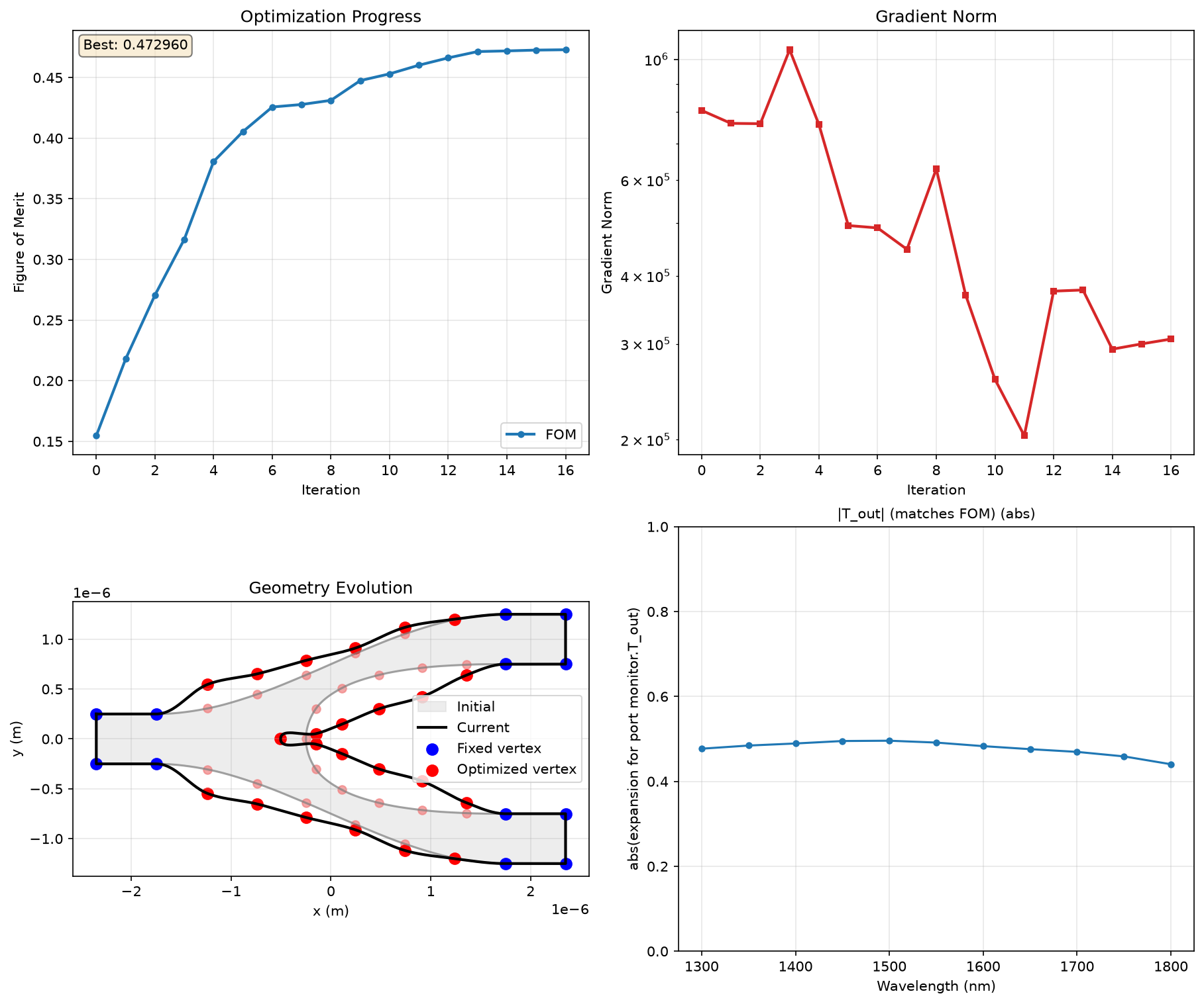
# Visualizer 1: FOM trace, gradient-norm trace, current geometry, and
# the real part of the Ey field so we can watch the splitter mode reshape
# during optimization.
# +
visualizer = lmpt.GraphicalVisualizer(
figsize=(12, 10),
layout=(2, 2), # Arrange panels in 2x2 grid
panels=[
lmpt.FomPanel(),
lmpt.GradientNormPanel(),
lmpt.GeometryPanel(),
lmpt.MonitorPanel(
monitor_name="FDTD::ports::port_out1",
result_name="expansion for port monitor.T_out",
operation="abs",
title="|T_out| (matches FOM)",
# Clamp the transmission trace to the physical
# [0, 1] range so the plot stays comparable
# iteration-to-iteration even when the
# baseline transmission starts very low.
# ``axes_kwargs`` is forwarded verbatim to
# ``ax.set(**axes_kwargs)``.
axes_kwargs={"ylim": (0.0, 1.0)},
),
],
)
# -
# + [markdown]
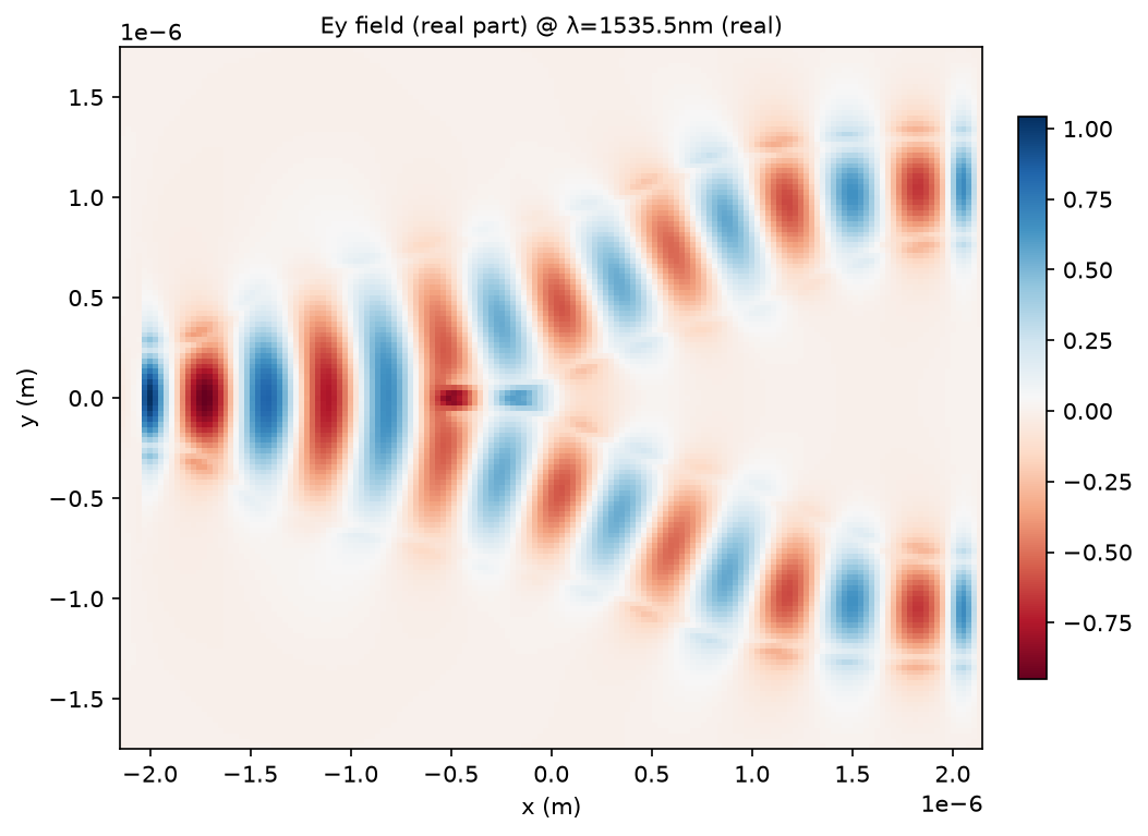
# Visualizer 2: Plot the y-direction electric field at the midplane monitor, for the midband wavelength.
# -
# +
visualizer2 = lmpt.GraphicalVisualizer(
filename_prefix="field_plot_Ey",
panels=[
lmpt.MonitorPanel(monitor_name="field_monitor", result_name="E.Ey", operation="real", title="Ey field (real part)"),
],
)
# -
# ### Optimization session
# Put everything together into an optimization session
optimization = lmpt.Optimization(
project=project,
optimizer=optimizer,
callbacks=[lmpt.FileLogger(), visualizer, visualizer2],
)
# ### Run optimization
result = optimization.run()
# + [markdown]
# The final visualizer is shown below
#  # The final electric field is shown below
#
# The final electric field is shown below
#  # -
# ## Save project
best_params, best_fom = result
project.save_project("y_branch_final.fsp", params=best_params)
# ## Export as gds
project_dir = Path(project.fom.config_map.project_folder).resolve()
with lumapi.FDTD(project=str(project_dir / "y_branch_final.fsp"), hide=True) as fdtd:
f = fdtd.gdsopen(str(project_dir / "y_branch_final.gds"))
fdtd.gdsbegincell(f, "y_branch")
# Material is set to the index as it was created as an "
# -
# ## Save project
best_params, best_fom = result
project.save_project("y_branch_final.fsp", params=best_params)
# ## Export as gds
project_dir = Path(project.fom.config_map.project_folder).resolve()
with lumapi.FDTD(project=str(project_dir / "y_branch_final.fsp"), hide=True) as fdtd:
f = fdtd.gdsopen(str(project_dir / "y_branch_final.gds"))
fdtd.gdsbegincell(f, "y_branch")
# Material is set to the index as it was created as an "