# # Photonic Crystal Bandstructure (FDTD)
#
# This example demonstrates a photonic crystal simulation utilizing Structure and Analysis Group objects.
# Based on: https://optics.ansys.com/hc/en-us/articles/360041566614-Rectangular-Photonic-Crystal-Bandstructure
#
#
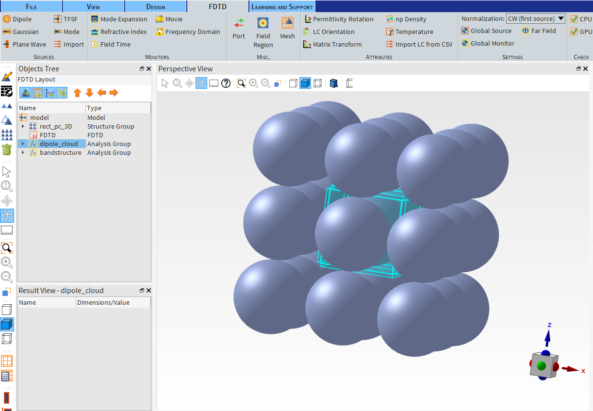
# In Part 1, we build the structure and set the FDTD simulation region.
# In this case, the spheres are holes (filled with air, n = 1) and the background material is a simple dielectric material.
# Some advanced simulation objects, including the dipole cloud source and bandstructure analysis groups, are imported from the Object Library.
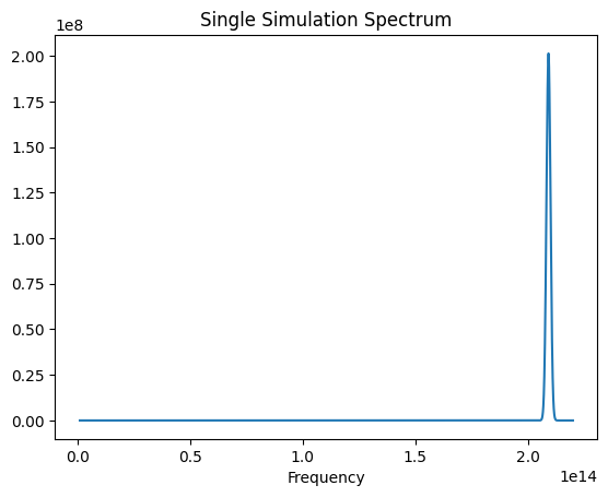
# We run a single simulation and visualize the resulting spectrum.
#
# In Part 2, we set up a series of sweeps to collect the resonant frequencies.
# In this example, we use the built-in sweep tool in Lumerical, but the parameter sweeps could also be set up from Python.
# We then run the sweeps and plot the results.
#
# Prerequisites: Valid FDTD license is required.
# Perform required imports
# +
from collections import OrderedDict
import itertools
import matplotlib.pyplot as plt # Only required for plotting
import numpy as np
import ansys.lumerical.core as lumapi
# -
# ## Part 1: Set up structures and simulation objects
#  # +
# Define parameters
# Set filename for saving and loading
filename = "photonic_crystal_bandstructure.fsp"
# set desired period of the array (3D)
ax = 0.5e-6
ay = 0.5e-6
az = 0.5e-6
# number of spheres in each direction
nx = 3
ny = 3
nz = 3
sphere_radius = 0.25e-6
sphere_index = 1 # Specify index if "Object defined dielectric" is used; otherwise, specify material from database below
sphere_material = "etch" # Etch n = 1 (air)
background_index = 3.6055
# Define frequencies / wavelengths of interest
f1 = 1e12 # THz
f2 = 220e12 # THz
# +
# Initialize session and build simulation objects. Set hide = True to hide the Lumerical GUI.
# This block will build an array of spheres for the photonic crystal structure.
# We add an FDTD region, sources, and monitors. The sources and monitors are imported from the Object Library.
# Finally, the simulation file is saved to the file name set earlier.
with lumapi.FDTD(hide=False) as fdtd:
# Add rectangular lattice array of spheres
# Note you can also use Lumerical's built-in "rect_pc_3D" object using fdtd.addobject("rect_pc_3D")
# In this example, we construct the array programmatically
fdtd.addstructuregroup({"name": "rect_pc_3D"})
for ix, iy, iz in itertools.product(*map(range, (nx, ny, nz))):
objname = f"c{ix}{iy}{iz}"
fdtd.addsphere(
{"name": objname, "x": (ix - 1) * ax, "y": (iy - 1) * ay, "z": (iz - 1) * az, "radius": sphere_radius, "material": sphere_material}
)
fdtd.addtogroup("rect_pc_3D") # Adds the recently created sphere to the structure group
# Add FDTD region
dx = 0.025e-6 # Mesh dx, dy, dz
fdtd_geometry_props = {"x": 0, "x span": ax, "y": 0, "y span": ay, "z": 0, "z span": az}
fdtd_mesh_props = {"index": background_index, "mesh type": "uniform", "dx": dx, "dy": dx, "dz": dx}
fdtd_boundary_props = {"x min bc": "Bloch", "y min bc": "Bloch", "z min bc": "Bloch", "set based on source angle": False, "bloch units": "SI"}
# Combine properties settings into one dictionary
fdtd_props = OrderedDict({**fdtd_geometry_props, **fdtd_mesh_props, **fdtd_boundary_props})
fdtd.addfdtd(properties=fdtd_props)
# Set up sources (dipole cloud) and monitors (bandstructure)
# These are both Analysis Groups available from the object library
dipole_geometry_props = {"n dipoles": 3, "lattice type": 3, "z span": az, "ax": ax, "ay": ay, "az": az, "a": az, "x": 0, "y": 0, "z": 0}
dipole_frequency_props = {"f1": f1, "f2": f2, "kx": 0.5, "ky": 0, "kz": 0}
dipole_props = OrderedDict({**dipole_geometry_props, **dipole_frequency_props})
fdtd.addobject("dipole_cloud", properties=dipole_props)
bandstructure_geometry_props = {"n monitors": 10, "x": 0, "x span": ax, "y": 0, "y span": ay, "z": 0, "z span": az}
bandstructure_frequency_props = {"f1": f1, "f2": f2}
bandstructure_props = OrderedDict({**bandstructure_geometry_props, **bandstructure_frequency_props})
fdtd.addobject("bandstructure", properties=bandstructure_props)
# zoom CAD view around simulation region
fdtd.select("FDTD")
fdtd.setview("extent")
fdtd.save(filename)
print("File saved to folder as: " + filename)
# +
# Open the file and run a single simulation. Visualize the spectrum.
with lumapi.FDTD(filename, hide=False) as fdtd:
print("Simulation running...")
fdtd.run()
print("Run completed. Analyzing and plotting results...")
fdtd.runanalysis()
# Plot results
single_spectrum = fdtd.getresult("bandstructure", "spectrum")
spectrum = single_spectrum["fd"]
frequencies = single_spectrum["f"]
plt.figure()
plt.plot(frequencies, spectrum)
plt.title("Single Simulation Spectrum")
plt.xlabel("Frequency")
plt.show(block=False)
plt.pause(2)
# -
#
# +
# Define parameters
# Set filename for saving and loading
filename = "photonic_crystal_bandstructure.fsp"
# set desired period of the array (3D)
ax = 0.5e-6
ay = 0.5e-6
az = 0.5e-6
# number of spheres in each direction
nx = 3
ny = 3
nz = 3
sphere_radius = 0.25e-6
sphere_index = 1 # Specify index if "Object defined dielectric" is used; otherwise, specify material from database below
sphere_material = "etch" # Etch n = 1 (air)
background_index = 3.6055
# Define frequencies / wavelengths of interest
f1 = 1e12 # THz
f2 = 220e12 # THz
# +
# Initialize session and build simulation objects. Set hide = True to hide the Lumerical GUI.
# This block will build an array of spheres for the photonic crystal structure.
# We add an FDTD region, sources, and monitors. The sources and monitors are imported from the Object Library.
# Finally, the simulation file is saved to the file name set earlier.
with lumapi.FDTD(hide=False) as fdtd:
# Add rectangular lattice array of spheres
# Note you can also use Lumerical's built-in "rect_pc_3D" object using fdtd.addobject("rect_pc_3D")
# In this example, we construct the array programmatically
fdtd.addstructuregroup({"name": "rect_pc_3D"})
for ix, iy, iz in itertools.product(*map(range, (nx, ny, nz))):
objname = f"c{ix}{iy}{iz}"
fdtd.addsphere(
{"name": objname, "x": (ix - 1) * ax, "y": (iy - 1) * ay, "z": (iz - 1) * az, "radius": sphere_radius, "material": sphere_material}
)
fdtd.addtogroup("rect_pc_3D") # Adds the recently created sphere to the structure group
# Add FDTD region
dx = 0.025e-6 # Mesh dx, dy, dz
fdtd_geometry_props = {"x": 0, "x span": ax, "y": 0, "y span": ay, "z": 0, "z span": az}
fdtd_mesh_props = {"index": background_index, "mesh type": "uniform", "dx": dx, "dy": dx, "dz": dx}
fdtd_boundary_props = {"x min bc": "Bloch", "y min bc": "Bloch", "z min bc": "Bloch", "set based on source angle": False, "bloch units": "SI"}
# Combine properties settings into one dictionary
fdtd_props = OrderedDict({**fdtd_geometry_props, **fdtd_mesh_props, **fdtd_boundary_props})
fdtd.addfdtd(properties=fdtd_props)
# Set up sources (dipole cloud) and monitors (bandstructure)
# These are both Analysis Groups available from the object library
dipole_geometry_props = {"n dipoles": 3, "lattice type": 3, "z span": az, "ax": ax, "ay": ay, "az": az, "a": az, "x": 0, "y": 0, "z": 0}
dipole_frequency_props = {"f1": f1, "f2": f2, "kx": 0.5, "ky": 0, "kz": 0}
dipole_props = OrderedDict({**dipole_geometry_props, **dipole_frequency_props})
fdtd.addobject("dipole_cloud", properties=dipole_props)
bandstructure_geometry_props = {"n monitors": 10, "x": 0, "x span": ax, "y": 0, "y span": ay, "z": 0, "z span": az}
bandstructure_frequency_props = {"f1": f1, "f2": f2}
bandstructure_props = OrderedDict({**bandstructure_geometry_props, **bandstructure_frequency_props})
fdtd.addobject("bandstructure", properties=bandstructure_props)
# zoom CAD view around simulation region
fdtd.select("FDTD")
fdtd.setview("extent")
fdtd.save(filename)
print("File saved to folder as: " + filename)
# +
# Open the file and run a single simulation. Visualize the spectrum.
with lumapi.FDTD(filename, hide=False) as fdtd:
print("Simulation running...")
fdtd.run()
print("Run completed. Analyzing and plotting results...")
fdtd.runanalysis()
# Plot results
single_spectrum = fdtd.getresult("bandstructure", "spectrum")
spectrum = single_spectrum["fd"]
frequencies = single_spectrum["f"]
plt.figure()
plt.plot(frequencies, spectrum)
plt.title("Single Simulation Spectrum")
plt.xlabel("Frequency")
plt.show(block=False)
plt.pause(2)
# -
#  # ## Part 2: Set up and run sweeps to extract resonant frequencies and plot the bandstructure
# +
# Normalization factor for SI units; see note above.
norm_x = 2 * np.pi / ax
norm_y = 2 * np.pi / ay
norm_z = 2 * np.pi / az
# The total number of simulations will be num_points*3
num_points = 5
# Define a function to add the sweeps
def add_bandstructure_sweep(sweep_name, x_start, x_stop, y_start, y_stop, z_start, z_stop):
"""Set up a sweep for bandstructure calculations."""
fdtd.addsweep()
fdtd.setsweep("sweep", "name", sweep_name)
fdtd.setsweep(sweep_name, "type", "Ranges")
fdtd.setsweep(sweep_name, "number of points", num_points)
# set the sweep properties
props_kx = {"Name": "kx", "Parameter": "::model::FDTD::kx", "Type": "Number", "Start": x_start, "Stop": x_stop}
fdtd.addsweepparameter(sweep_name, props_kx)
props_ky = {"Name": "ky", "Parameter": "::model::FDTD::ky", "Type": "Number", "Start": y_start, "Stop": y_stop}
fdtd.addsweepparameter(sweep_name, props_ky)
props_kz = {"Name": "kz", "Parameter": "::model::FDTD::kz", "Type": "Number", "Start": z_start, "Stop": z_stop}
fdtd.addsweepparameter(sweep_name, props_kz)
# define results
result_fs = {"Name": "fs", "Result": "::model::bandstructure::fs"}
fdtd.addsweepresult(sweep_name, result_fs)
result_spectrum = {"Name": "fs", "Result": "::model::bandstructure::spectrum"}
fdtd.addsweepresult(sweep_name, result_spectrum)
# Now add the sweeps to the file
with lumapi.FDTD(filename, hide=False) as fdtd:
# Add Gamma-X sweep
add_bandstructure_sweep("Gamma-X", 0 * norm_x, 0.5 * norm_x, 0 * norm_y, 0 * norm_y, 0 * norm_z, 0 * norm_z)
# Add X-M sweep
add_bandstructure_sweep("X-M", 0.5 * norm_x, 0.5 * norm_x, 0 * norm_y, 0.5 * norm_y, 0 * norm_z, 0 * norm_z)
# Add M-R sweep
add_bandstructure_sweep("M-R", 0.5 * norm_x, 0.5 * norm_x, 0.5 * norm_y, 0.5 * norm_y, 0 * norm_z, 0.5 * norm_z)
fdtd.save(filename)
print("Sweeps have been set up.")
# -
# Now run all the sweeps - this may take a few minutes
with lumapi.FDTD(filename, hide=False) as fdtd:
print("Running sweeps...")
fdtd.runsweep()
fdtd.save(filename)
# If you have previously run the sweeps, you can load them using this line instead:
# fdtd.loadsweep()
print("Sweeps have been run.")
# Retrieve and analyze data from the sweeps
with lumapi.FDTD(filename, hide=False) as fdtd:
fs_all = np.zeros((50, 3 * num_points)) # 50 is the number of frequencies, and there are 3*num_points bandstructure points
sweepname = "Gamma-X"
resonance = fdtd.getsweepresult(sweepname, "fs") # Results are returned as Python dict
resonance_fs = resonance["fs"]
fs_all[0:50, 0:num_points] = resonance_fs
sweepname = "X-M"
resonance = fdtd.getsweepresult(sweepname, "fs") # Results are returned as Python dict
resonance_fs = resonance["fs"]
fs_all[0:50, num_points : 2 * num_points] = resonance_fs
sweepname = "M-R"
resonance = fdtd.getsweepresult(sweepname, "fs") # Results are returned as Python dict
resonance_fs = resonance["fs"]
fs_all[0:50, 2 * num_points : 3 * num_points] = resonance_fs
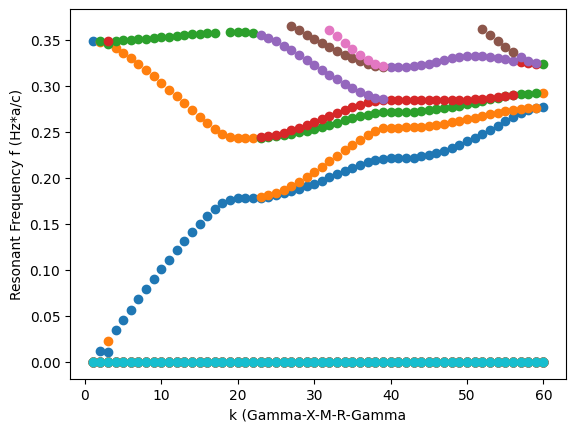
k = np.linspace(1, 3 * num_points, 3 * num_points)
c = 3 * 10**8
plt.figure()
for f in range(0, 50):
plt.scatter(k, fs_all[f] * ax / c)
plt.xlabel("k (Gamma-X-M-R-Gamma")
plt.ylabel("Resonant Frequency f (Hz*a/c)")
plt.show(block=False)
plt.pause(10)
#
# ## Part 2: Set up and run sweeps to extract resonant frequencies and plot the bandstructure
# +
# Normalization factor for SI units; see note above.
norm_x = 2 * np.pi / ax
norm_y = 2 * np.pi / ay
norm_z = 2 * np.pi / az
# The total number of simulations will be num_points*3
num_points = 5
# Define a function to add the sweeps
def add_bandstructure_sweep(sweep_name, x_start, x_stop, y_start, y_stop, z_start, z_stop):
"""Set up a sweep for bandstructure calculations."""
fdtd.addsweep()
fdtd.setsweep("sweep", "name", sweep_name)
fdtd.setsweep(sweep_name, "type", "Ranges")
fdtd.setsweep(sweep_name, "number of points", num_points)
# set the sweep properties
props_kx = {"Name": "kx", "Parameter": "::model::FDTD::kx", "Type": "Number", "Start": x_start, "Stop": x_stop}
fdtd.addsweepparameter(sweep_name, props_kx)
props_ky = {"Name": "ky", "Parameter": "::model::FDTD::ky", "Type": "Number", "Start": y_start, "Stop": y_stop}
fdtd.addsweepparameter(sweep_name, props_ky)
props_kz = {"Name": "kz", "Parameter": "::model::FDTD::kz", "Type": "Number", "Start": z_start, "Stop": z_stop}
fdtd.addsweepparameter(sweep_name, props_kz)
# define results
result_fs = {"Name": "fs", "Result": "::model::bandstructure::fs"}
fdtd.addsweepresult(sweep_name, result_fs)
result_spectrum = {"Name": "fs", "Result": "::model::bandstructure::spectrum"}
fdtd.addsweepresult(sweep_name, result_spectrum)
# Now add the sweeps to the file
with lumapi.FDTD(filename, hide=False) as fdtd:
# Add Gamma-X sweep
add_bandstructure_sweep("Gamma-X", 0 * norm_x, 0.5 * norm_x, 0 * norm_y, 0 * norm_y, 0 * norm_z, 0 * norm_z)
# Add X-M sweep
add_bandstructure_sweep("X-M", 0.5 * norm_x, 0.5 * norm_x, 0 * norm_y, 0.5 * norm_y, 0 * norm_z, 0 * norm_z)
# Add M-R sweep
add_bandstructure_sweep("M-R", 0.5 * norm_x, 0.5 * norm_x, 0.5 * norm_y, 0.5 * norm_y, 0 * norm_z, 0.5 * norm_z)
fdtd.save(filename)
print("Sweeps have been set up.")
# -
# Now run all the sweeps - this may take a few minutes
with lumapi.FDTD(filename, hide=False) as fdtd:
print("Running sweeps...")
fdtd.runsweep()
fdtd.save(filename)
# If you have previously run the sweeps, you can load them using this line instead:
# fdtd.loadsweep()
print("Sweeps have been run.")
# Retrieve and analyze data from the sweeps
with lumapi.FDTD(filename, hide=False) as fdtd:
fs_all = np.zeros((50, 3 * num_points)) # 50 is the number of frequencies, and there are 3*num_points bandstructure points
sweepname = "Gamma-X"
resonance = fdtd.getsweepresult(sweepname, "fs") # Results are returned as Python dict
resonance_fs = resonance["fs"]
fs_all[0:50, 0:num_points] = resonance_fs
sweepname = "X-M"
resonance = fdtd.getsweepresult(sweepname, "fs") # Results are returned as Python dict
resonance_fs = resonance["fs"]
fs_all[0:50, num_points : 2 * num_points] = resonance_fs
sweepname = "M-R"
resonance = fdtd.getsweepresult(sweepname, "fs") # Results are returned as Python dict
resonance_fs = resonance["fs"]
fs_all[0:50, 2 * num_points : 3 * num_points] = resonance_fs
k = np.linspace(1, 3 * num_points, 3 * num_points)
c = 3 * 10**8
plt.figure()
for f in range(0, 50):
plt.scatter(k, fs_all[f] * ax / c)
plt.xlabel("k (Gamma-X-M-R-Gamma")
plt.ylabel("Resonant Frequency f (Hz*a/c)")
plt.show(block=False)
plt.pause(10)
#