

Installation and getting started#
Installation#

You can install PyLumerical using pip.
First, create a virtual environment and activate it to avoid dependency conflicts and to keep your global Python environment clean.
Note
If you have multiple Python versions installed, ensure you are using the right executable for the virtual environment. The supported Python versions are at the top of this page.
1python -m venv .venv
2source .venv/bin/activate
1python -m venv .venv
2.venv\\Scripts\\activate.bat
1python -m venv .venv
2.venv\\Scripts\\Activate.ps1
Then, upgrade pip to the latest version, and install PyLumerical with the package name ansys-lumerical-core.
1python -m pip install -U pip
2python -m pip install ansys-lumerical-core
Tip
Using a virtual environment isn’t a requirement, but it’s a best practice for Python development. PyLumerical is compatible with various Python IDEs including VS Code, Jupyter Notebook, and Cursor. After installation, you can use your preferred editor to start using PyLumerical. Refer to the documentation of your IDE for instructions on how to use the virtual environment.
Requirements#
You must have an Ansys Lumerical GUI license along with Lumerical 2022 R1 or later on your computer to use PyLumerical. For more information, please visit the licensing page on the Ansys Optics website.
Upon importing PyLumerical, the autodiscovery logic automatically locates the Lumerical installation path and configures interop.
If autodiscovery fails, set the LUMERICAL_HOME environment variable before import and start a new Python session.
To use the Lumerical photonic inverse design module lumopt2, you must have Ansys Lumerical FDTD™ version 2026 R1.2 or later installed on your computer. The autodiscovery logic automatically locates the lumopt2 module if it is available.
Importing modules#
To use PyLumerical for simulation automation:
1import ansys.lumerical.core as lumapi
Tip
When imported this way, you can directly use your scripts written with the legacy lumapi Python module.
To use the lumopt2 inverse design module, use the code below. For further information, see the lumopt2 introduction page.
1import ansys.lumerical.core.lumopt2 as lmpt
Warning
To ensure correct functionality, only import
lumopt2throughansys.lumerical.core.Manual
sys.pathoverrides forlumopt2are unsupported. Thelumopt2module bundled with Ansys Lumerical products silently takes precedence over those added tosys.path.
My first PyLumerical project#
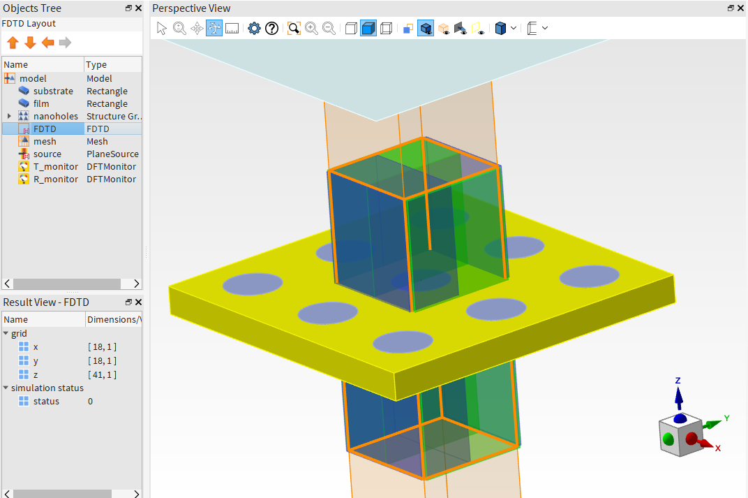
The code snippet below provides a simple project of using PyLumerical to drive a Lumerical FDTD simulation with an array of nanoholes on a gold film atop a glass substrate.
Step 1 - Import and simulation parameters
Import PyLumerical and define various simulation parameters.
Show imports
1
2from collections import OrderedDict
3
4import matplotlib.pyplot as plt
5
6import ansys.lumerical.core as lumapi
7
Show parameter definition
 1# Define parameters
 2
 3filename = "Nanohole_array.fsp"
 4
 5# Parameters related to the patterned film
 6periodicity = 400e-9  # 400 nm periodic array
 7film_thickness = 100e-9
 8hole_radius = 100e-9  # radius of the nanoholes
 9nx = ny = 3  # Number of nanoholes
10
11# Parameters for the substrate
12substrate_thickness = 1e-6
13substrate_span = 1.2e-6
14
15# FDTD region and mesh
16fdtd_z_span = 1e-6  # Ensure span is large enough to capture both T, R monitors
17transmission_z = 0.4e-6  # z position of top "T" monitor
18reflection_z = -0.2e-6  # z position of bottom "R" monitor
19dx = 0.01e-6  # mesh override resolution
20
21# Source and wavelengths
22source_z = 0.3e-6  # position of source
23wavelength_start = 0.4e-6
24wavelength_stop = 0.7e-6
Step 2 - Build simulation
Set up the simulation, including the region, geometry, materials, source, and monitors.
Show simulation setup
 1# Initialize session and build simulation objects. Set hide = True to hide the Lumerical GUI.
 2
 3with lumapi.FDTD(hide=False) as fdtd:
 4    # Add the substrate
 5    fdtd.addrect(name="substrate",
 6                 x_span=substrate_span,
 7                 y_span=substrate_span,
 8                 z_max=0,
 9                 z_min=substrate_thickness,
10                 material="SiO2 (Glass) - Palik")
11
12    # Add the gold film
13    fdtd.addrect(name="film",
14                 x_span=substrate_span,
15                 y_span=substrate_span,
16                 z_max=film_thickness,
17                 z_min=0,
18                 material="Au (Gold) - CRC")
19
20    # Add the nanohole array in the gold layer
21    # For this, we use the built-in rectangular photonic crystal object from the library
22    pc_props = {
23        "name": "nanoholes",
24        "material": "etch",
25        "radius": hole_radius,
26        "z": film_thickness / 2,
27        "z span": film_thickness,
28        "nx": nx,
29        "ny": ny,
30        "ax": periodicity,
31        "ay": periodicity,
32    }
33    fdtd.addobject("rect_pc")
34    fdtd.set(pc_props)
35
36    # Set up the simulation region
37    fdtd_geometry_props = {"x": 0, "x span": periodicity, "y": 0, "y span": periodicity, "z": 0, "z span": fdtd_z_span}
38    # Use symmetric boundary conditions in x and y and steep angle PML profile in z
39    fdtd_boundary_props = {
40        "allow symmetry on all boundaries": 1,
41        "x min bc": "anti-symmetric",
42        "x max bc": "anti-symmetric",
43        "y min bc": "symmetric",
44        "y max bc": "symmetric",
45        "z min bc": "PML",
46        "z max bc": "PML",
47        "pml profile": 3,
48    }
49    # Combine properties settings into one dictionary
50    fdtd_props = OrderedDict({**fdtd_geometry_props, **fdtd_boundary_props})
51    fdtd.addfdtd(properties=fdtd_props)
52
53    # Add a mesh override region around the holes
54    fdtd.addmesh(dx=dx, dy=dx, dz=dx, based_on_a_structure=1, structure="circle")
55
56    # Add plane wave source
57    fdtd.addplane(injection_axis="z-axis", direction="backward", x_span=substrate_span, y_span=substrate_span, z=source_z)
58    fdtd.setglobalsource("wavelength start", wavelength_start)
59    fdtd.setglobalsource("wavelength stop", wavelength_stop)
60
61    # Set up frequency domain monitors to measure R and T
62    # First, set global monitor properties
63    # Source limits will be used by default to define min/max wavelength
64    fdtd.setglobalmonitor("frequency points", 50)
65    # Now add the monitors
66    fdtd.adddftmonitor(name="T_monitor",
67                       monitor_type="2D Z-normal",
68                       x_span=substrate_span,
69                       y_span=substrate_span,
70                       z=transmission_z)
71    fdtd.adddftmonitor(name="R_monitor",
72                       monitor_type="2D Z-normal",
73                       x_span=substrate_span,
74                       y_span=substrate_span,
75                       z=reflection_z)
76
77    # zoom CAD view around simulation region
78    fdtd.select("FDTD")
79    fdtd.setview("extent")
80
81    fdtd.save(filename)
82    print("File saved to folder as: " + filename)
The simulation file is saved in the current working directory - you can open it in the Lumerical GUI to check the simulation setup.
Step 3 - Run and plot results
Run the simulation and plot the transmission and reflection spectra.
Show simulation run and plotting
 1# Open the file and run the simulation! Visualize the T/R spectrum.
 2with lumapi.FDTD(filename, hide=True) as fdtd:
 3    print("Starting simulation now...")
 4    fdtd.run()
 5    print("Run completed.")
 6
 7    # Retrieve results
 8    T = fdtd.getresult("T_monitor", "T")  # Returns lumerical dataset T vs lambda/f
 9    R = fdtd.getresult("R_monitor", "T")
10
11    # Visualize using matplotlib
12    fig, ax = plt.subplots()
13    ax.plot(T["lambda"] * 1e9, T["T"], label="Transmission")
14    ax.plot(R["lambda"] * 1e9, -1 * R["T"], label="Reflection")  # light traveling along -z so T result is negative
15    ax.set_xlabel("Wavelength [nm]")
16    ax.set_ylabel("T/R")
17    ax.legend()
18    plt.show()
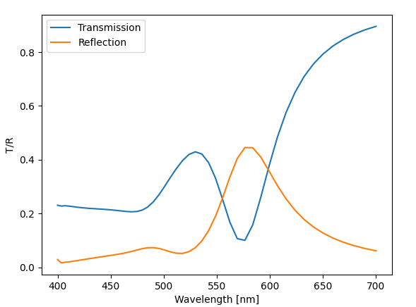
The figure below shows the transmission and reflection spectrum of the array.
Full script
Show full script for copy and paste
  1# --- Imports ---
  2
  3from collections import OrderedDict
  4
  5import matplotlib.pyplot as plt
  6
  7import ansys.lumerical.core as lumapi
  8
  9# --- Imports end ---
 10
 11# --- Parameters ---
 12# Define parameters
 13
 14filename = "Nanohole_array.fsp"
 15
 16# Parameters related to the patterned film
 17periodicity = 400e-9  # 400 nm periodic array
 18film_thickness = 100e-9
 19hole_radius = 100e-9  # radius of the nanoholes
 20nx = ny = 3  # Number of nanoholes
 21
 22# Parameters for the substrate
 23substrate_thickness = 1e-6
 24substrate_span = 1.2e-6
 25
 26# FDTD region and mesh
 27fdtd_z_span = 1e-6  # Ensure span is large enough to capture both T, R monitors
 28transmission_z = 0.4e-6  # z position of top "T" monitor
 29reflection_z = -0.2e-6  # z position of bottom "R" monitor
 30dx = 0.01e-6  # mesh override resolution
 31
 32# Source and wavelengths
 33source_z = 0.3e-6  # position of source
 34wavelength_start = 0.4e-6
 35wavelength_stop = 0.7e-6
 36# --- Parameters end ---
 37
 38# --- Simulation setup ---
 39# Initialize session and build simulation objects. Set hide = True to hide the Lumerical GUI.
 40
 41with lumapi.FDTD(hide=False) as fdtd:
 42    # Add the substrate
 43    fdtd.addrect(name="substrate",
 44                 x_span=substrate_span,
 45                 y_span=substrate_span,
 46                 z_max=0,
 47                 z_min=substrate_thickness,
 48                 material="SiO2 (Glass) - Palik")
 49
 50    # Add the gold film
 51    fdtd.addrect(name="film",
 52                 x_span=substrate_span,
 53                 y_span=substrate_span,
 54                 z_max=film_thickness,
 55                 z_min=0,
 56                 material="Au (Gold) - CRC")
 57
 58    # Add the nanohole array in the gold layer
 59    # For this, we use the built-in rectangular photonic crystal object from the library
 60    pc_props = {
 61        "name": "nanoholes",
 62        "material": "etch",
 63        "radius": hole_radius,
 64        "z": film_thickness / 2,
 65        "z span": film_thickness,
 66        "nx": nx,
 67        "ny": ny,
 68        "ax": periodicity,
 69        "ay": periodicity,
 70    }
 71    fdtd.addobject("rect_pc")
 72    fdtd.set(pc_props)
 73
 74    # Set up the simulation region
 75    fdtd_geometry_props = {"x": 0, "x span": periodicity, "y": 0, "y span": periodicity, "z": 0, "z span": fdtd_z_span}
 76    # Use symmetric boundary conditions in x and y and steep angle PML profile in z
 77    fdtd_boundary_props = {
 78        "allow symmetry on all boundaries": 1,
 79        "x min bc": "anti-symmetric",
 80        "x max bc": "anti-symmetric",
 81        "y min bc": "symmetric",
 82        "y max bc": "symmetric",
 83        "z min bc": "PML",
 84        "z max bc": "PML",
 85        "pml profile": 3,
 86    }
 87    # Combine properties settings into one dictionary
 88    fdtd_props = OrderedDict({**fdtd_geometry_props, **fdtd_boundary_props})
 89    fdtd.addfdtd(properties=fdtd_props)
 90
 91    # Add a mesh override region around the holes
 92    fdtd.addmesh(dx=dx, dy=dx, dz=dx, based_on_a_structure=1, structure="circle")
 93
 94    # Add plane wave source
 95    fdtd.addplane(injection_axis="z-axis", direction="backward", x_span=substrate_span, y_span=substrate_span, z=source_z)
 96    fdtd.setglobalsource("wavelength start", wavelength_start)
 97    fdtd.setglobalsource("wavelength stop", wavelength_stop)
 98
 99    # Set up frequency domain monitors to measure R and T
100    # First, set global monitor properties
101    # Source limits will be used by default to define min/max wavelength
102    fdtd.setglobalmonitor("frequency points", 50)
103    # Now add the monitors
104    fdtd.adddftmonitor(name="T_monitor",
105                       monitor_type="2D Z-normal",
106                       x_span=substrate_span,
107                       y_span=substrate_span,
108                       z=transmission_z)
109    fdtd.adddftmonitor(name="R_monitor",
110                       monitor_type="2D Z-normal",
111                       x_span=substrate_span,
112                       y_span=substrate_span,
113                       z=reflection_z)
114
115    # zoom CAD view around simulation region
116    fdtd.select("FDTD")
117    fdtd.setview("extent")
118
119    fdtd.save(filename)
120    print("File saved to folder as: " + filename)
121# --- Simulation setup end --
122
123
124# --- Run ---
125# Open the file and run the simulation! Visualize the T/R spectrum.
126with lumapi.FDTD(filename, hide=True) as fdtd:
127    print("Starting simulation now...")
128    fdtd.run()
129    print("Run completed.")
130
131    # Retrieve results
132    T = fdtd.getresult("T_monitor", "T")  # Returns lumerical dataset T vs lambda/f
133    R = fdtd.getresult("R_monitor", "T")
134
135    # Visualize using matplotlib
136    fig, ax = plt.subplots()
137    ax.plot(T["lambda"] * 1e9, T["T"], label="Transmission")
138    ax.plot(R["lambda"] * 1e9, -1 * R["T"], label="Reflection")  # light traveling along -z so T result is negative
139    ax.set_xlabel("Wavelength [nm]")
140    ax.set_ylabel("T/R")
141    ax.legend()
142    plt.show()
143# --- Run end ---
Further resources#
Information on key concepts of PyLumerical.
Reference for the PyLumerical API.
Gallery of examples using PyLumerical.
Reference for Lumerical scripting commands.
Introduction to using lumopt2 for photonic inverse design.
Recommended examples#
Recommended examples to further build your understanding of PyLumerical and its capabilities.
Run an FDTD simulation using PyLumerical and plot the electric field.
Run a waveguide simulation in MODE.
Run an an INTERCONNECT simulation for a ring resonator.