Basic FDTD Simulation - Python style commands#
A simple example to demonstrate using PyLumerical.
Sets up and runs a basic FDTD simulation. E field results are plotted using Matplotlib Demonstrates initializing objects using keyword arguments and OrderedDict.
Prerequisites:#
Valid FDTD license is required.
Perform required imports#
[ ]:
1from collections import OrderedDict
2
3import matplotlib.pyplot as plt
4
5import ansys.lumerical.core as lumapi
Open interactive session with the “with” context manager, run session, retrieve and plots results, and close session#
[ ]:
6# Set hide = True to hide the Lumerical GUI.
7with lumapi.FDTD() as fdtd:
8 # Set up simulation region using keyword arguments
9 fdtd.addfdtd(x=0, x_span=8e-6, y=0, y_span=8e-6, z=0.25e-6, z_span=0.5e-6)
10
11 # Set up source using Python OrderedDict
12 # OrderedDict is recommended when order is important
13 # Here, the scalar appproximation prop should be set before waist radius
14 props = OrderedDict(
15 [
16 ("injection axis", "z"),
17 ("direction", "forward"),
18 ("x", 0),
19 ("x span", 16e-6),
20 ("y", 0),
21 ("y span", 16e-6),
22 ("z", 0.2e-6),
23 ("use scalar approximation", 1),
24 ("waist radius w0", 2e-6),
25 ("distance from waist", 0),
26 ("wavelength start", 1e-6),
27 ("wavelength stop", 1e-6),
28 ]
29 )
30 fdtd.addgaussian(properties=props)
31
32 # Set up monitor using regular dict
33 props = {"monitor type": "2D Z-normal", "x": 0, "x span": 16e-6, "y": 0, "y span": 16e-6, "z": 0.3e-6}
34 fdtd.adddftmonitor(properties=props)
35
36 # Run and save simulation
37 fdtd.save("fdtd_tutorial.fsp")
38 fdtd.run()
39
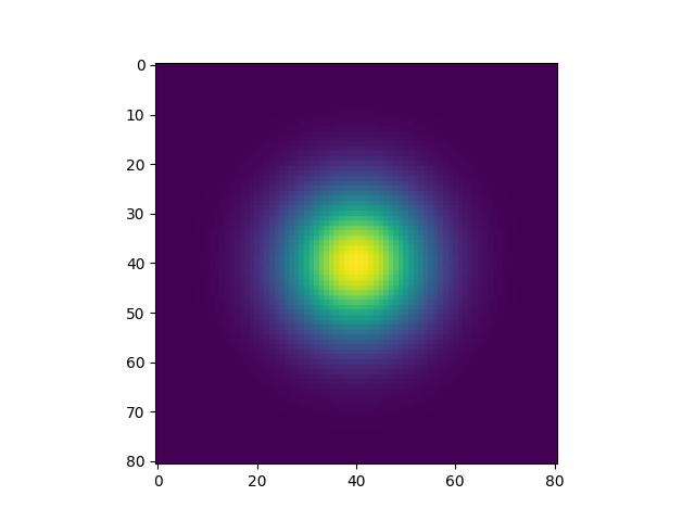
40 # Retrieve and plot results
41 E2 = fdtd.getelectric("monitor")[:, :, 0, 0]
42
43 plt.figure()
44 plt.imshow(E2)
45 plt.show()
46
47 print("Example complete. Press Enter to close.")
48 input()