Simple Waveguide (MODE FDE)#
A simple example using MODE. Waveguide (FDE): https://optics.ansys.com/hc/en-us/articles/360042800453-Waveguide-FDE
The Finite Difference Eigenmode (FDE) solver in MODE is used to characterize a straight waveguide.
In Part 1, we build the structure and set the FDE simulation region. In Part 2, we calculate the supported mode profiles of the waveguide.
Prerequisites: Valid MODE license is required.
Perform required imports
[ ]:
1from collections import OrderedDict
[ ]:
2import matplotlib.pyplot as plt
3import numpy as np
[ ]:
4import ansys.lumerical.core as lumapi
Part 1: Set up structures and simulation objects#
[ ]:
 5# Set hide = True to hide the Lumerical GUI.
 6mode = lumapi.MODE(hide=False)
 7
 8# Set key parameters
 9wavelength = 1.55e-6  # Center wavelength
10# Set the waveguide cross-section and material
11wg_width = 0.5e-6
12wg_height = 0.22e-6
13wg_material = "Si (Silicon) - Palik"
14# Set substrate and cladding cross-section and material
15sub_width = 10e-6
16sub_height = 5e-6
17sub_material = "SiO2 (Glass) - Palik"
18clad_width = 10e-6
19clad_height = 5e-6
20clad_material = "SiO2 (Glass) - Palik"
21# Set FDE region
22fde_x_span = 3e-6
23fde_y_span = 3e-6
24fde_y_center = wg_height / 2
25fde_z = 0e-6
26
27z_span = 1.0e-6  # Sets z span for all structures, but note FDE solver utilizes a cross section
28
29# Build substrate and cladding
30mode.addrect(name="substrate", x=0, x_span=sub_width, y_min=-sub_height, y_max=0, z=0, z_span=z_span, material=sub_material)
31mode.addrect(name="clad", x=0, x_span=clad_width, y_min=0, y_max=clad_height, z=0, z_span=z_span, material=clad_material)
[ ]:
32# Build waveguide
33# Use mesh order override to ensure waveguide object is prioritized over substrate and cladding
34wg_props = OrderedDict(
35    [
36        ("name", "waveguide"),
37        ("x", 0),
38        ("x span", wg_width),
39        ("y min", 0),
40        ("y max", wg_height),
41        ("z", 0),
42        ("z span", z_span),
43        ("material", wg_material),
44        ("override mesh order from material database", True),
45        ("mesh order", 1),
46    ]
47)
48mode.addrect(properties=wg_props)
[ ]:
49# Add FDE solver region
50fde_props = OrderedDict([("x", 0), ("x span", fde_x_span), ("y", fde_y_center), ("y span", fde_y_span), ("z", fde_z)])
51mode.addfde(properties=fde_props)
[ ]:
52# Add mesh override region
53mesh_props = OrderedDict(
54 [
55 ("set maximum mesh step", True),
56 ("override x mesh", True),
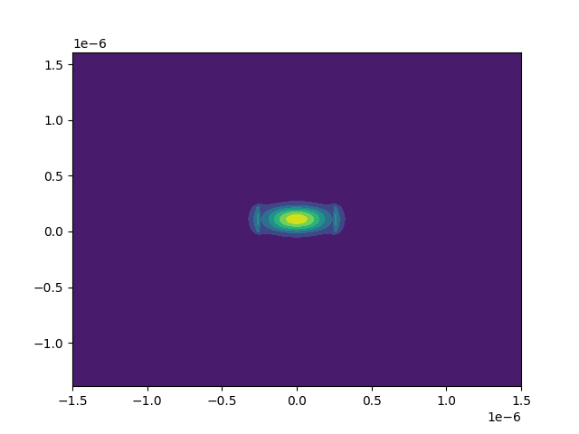
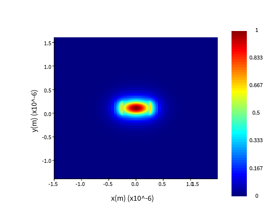
57 ("override y mesh", True),
58 ("dx", 0.01e-6),
59 ("dy", 0.01e-6),
60 ("based on a structure", True),
61 ("structure", "waveguide"),
62 ]
63)
64mode.addmesh(properties=mesh_props)
Part 2: Calculate the supported modes of the waveguide#
The analysis_props are equivalent to the settings in the Eigensolver Analysis window in the GUI.
[ ]:
65mode.setanalysis("wavelength", wavelength)
66mode.setanalysis("number of trial modes", 10)
67mode.setanalysis("search", "near n")
68mode.setanalysis("use max index", True)
[ ]:
69mode.findmodes()
[ ]:
70# Select and plot the fundamental mode
71selected_mode_number = 1
72selected_mode = "mode" + str(selected_mode_number)
73Efield = mode.getresult("FDE::data::" + selected_mode, "E")
74
75# Plot in Lumerical GUI
76mode.visualize((Efield))
[ ]:
77# Plot in Python - requires matplotlib
78# Note that Lumerical uses an unstructured mesh, so the spacing between points may be non-constant.
79# Therefore, it is preferable to collect x, y data from the monitor and plot using contourf.
80x, y = Efield["x"], Efield["y"]
81Ex, Ey, Ez = Efield["E"][:, :, 0, 0, 0], Efield["E"][:, :, 0, 0, 1], Efield["E"][:, :, 0, 0, 2]
82E_mag = np.abs(Ex) ** 2 + np.abs(Ey) ** 2 + np.abs(Ez) ** 2
83X, Y = np.meshgrid(x, y)  # Create meshgrid for plotting
84plt.figure()
85plt.contourf(X, Y, np.transpose(E_mag))
86plt.show()